rm(list = ls())
library(tidyverse)  # For tibble, ggplot2, etc.
library(broom) # Loaded just for the tidy() commandEstimate the Average Treatment Effect by Simple OLS
Statistical Methods for Causal Inference and Prediction (TPM039A)
teaching
TPM039A
Introduction
This lecture note simulates potential outcomes, randomly assigns treatment, and estimates the average treatment effect (ATE) by simple ordinary least squares (OLS) regression. It generates many samples and runs many regressions to demonstrate that the OLS estimator is correct on average – under random assignment, the simple OLS estimator is unbiased for the ATE.
Refer to JW (2025, Section 2.6) for background on regression with a binary x-variable. Refer to JW (2025, Section 2.7) for background on the potential outcomes framework and regression in an experimental setting.
Recall that unbiasedness means that the expected value of the estimator equals the estimand. JW does not use the term estimand, but we use it in this course. The estimand is the target parameter, the parameter we want to estimate. In our case, the estimator is the OLS slope coefficient on the treatment variable (\(\hat{\beta}_1\)), and the estimand is the ATE (\(\tau_{ATE}\)). Unbiasedness means: \[E[\hat{\beta}_1] = \tau_{ATE}\]
JW proves unbiasedness using mathematics – we demonstrate unbiasedness using simulation.
In this lecture note and in the rest of the course, I will not explain every R function and line of code. To learn R (or Python), consult Florian Heiss and Daniel Brunner’s coding supplement (www.urfie.net).
Setup
Clean the environment and load packages:
Simulate Data
We write a function to generate a tibble with \(n\) data points. A tibble is the tidyverse’s version of a data frame. It is similar to a data frame but has some nice features, e.g., it prints better in the console.
# Function to generate sample of size n
gen_sampl <- function(n = 100) {
  sampl <- tibble(
    y0 = rnorm(n, 40, 12),  # Potential outcome in untreated state
    tau = -10,              # Treatment effect
    y1 = y0 + tau,          # Potential outcome in treated state
    t = rbinom(n, 1, 0.5),  # Treatment assignment
    y = (1 - t)*y0 + t*y1   # Observed outcome
  )
  return(sampl)
}
We generate the data by calling the function gen_sampl(). The default sample size is 100, but we can change it by passing a different value to the function.
The data is generated as follows:
y0, the potential outcome under the control condition, is drawn from a normal distribution with mean 40 and standard deviation 12. We could have used any other distribution, e.g., uniform, exponential, etc.
tau, the individual treatment effect, is constant at -10. This choice encodes what Wooldridge calls the constant treatment effect assumption (Wooldridge, 2025, Section 2-7). If the individual treatment effect is the same for all units and equal to -10, by implication, the average treatment effect is also -10.
y1, the potential outcome under the treatment condition, is the sum of y0 and tau. This is obvious, right? Recall that the individual treatment effect is defined as the difference between the potential outcomes (\(\tau_i = Y_i(1) - Y_i(0)\)).
t, the treatment variable, is drawn from a Bernoulli distribution with probability 0.5, i.e., each unit has a 50% chance of being treated. This is a coin flip, which is one way of randomly assigning the treatment.
y, the observed outcome, is determined by the switching equation. If a unit is treated (t=1), we observe y1; if a unit is untreated (t=0), we observe y0.
We check that the function works by generating a sample of size 5 and printing it to the console.
# Generate one sample and show data
mydata <- gen_sampl(5)
mydata
# A tibble: 5 × 5
y0 tau y1 t y
<dbl> <dbl> <dbl> <int> <dbl>
1 27.7 -10 17.7 0 27.7
2 28.3 -10 18.3 0 28.3
3 50.2 -10 40.2 0 50.2
4 37.8 -10 27.8 0 37.8
5 64.3 -10 54.3 0 64.3We can see that the data has been generated as intended.
Now we generate r samples of size n and store them in a list. In R, a list is a data structure that can hold multiple objects, even of different types. Here, we use it to store many tibbles.
We need to create an empty list first, before filling it with content.
# Generate r samples of n data points
mydata <- list()  # Initialize list
r <- 1000         # Number of samples
n <- 30           # Sample size

# Set seed for reproducibility
set.seed(12345)

# Loop from 1 to r, storing r samples
for(j in 1:r) {
  mydata[[j]] <- gen_sampl(n)
}
Our function, gen_sampl(), creates a sample. The for-loop creates r samples and stores them as elements of the list mydata.
We print the first sample (list element) to verify that the loop does what it’s supposed to be doing.
mydata[[1]] # A tibble: 30 × 5
y0 tau y1 t y
<dbl> <dbl> <dbl> <int> <dbl>
1 47.0 -10 37.0 1 37.0
2 48.5 -10 38.5 0 48.5
3 38.7 -10 28.7 1 28.7
4 34.6 -10 24.6 1 24.6
5 47.3 -10 37.3 1 37.3
6 18.2 -10 8.18 0 18.2
7 47.6 -10 37.6 1 37.6
8 36.7 -10 26.7 0 36.7
9 36.6 -10 26.6 1 26.6
10 29.0 -10 19.0 1 19.0
# ℹ 20 more rowsRun Regressions
We will run r regressions, one for each sample. But for now, we run a regression using the first sample only and store the result in the object myreg. Then we print the result using the base R summary function.
myreg <- lm(y ~ t, data = mydata[[1]])
summary(myreg)
Call:
lm(formula = y ~ t, data = mydata[[1]])

Residuals:
    Min      1Q  Median      3Q     Max
-18.717  -7.478   2.268   6.552  24.759

Coefficients:
            Estimate Std. Error t value Pr(>|t|)
(Intercept)   36.902      3.157   11.69 2.76e-12 ***
t             -3.260      4.076   -0.80     0.43
---
Signif. codes:  0 '***' 0.001 '**' 0.01 '*' 0.05 '.' 0.1 ' ' 1

Residual standard error: 10.94 on 28 degrees of freedom
Multiple R-squared:  0.02234,   Adjusted R-squared:  -0.01257
F-statistic: 0.6399 on 1 and 28 DF,  p-value: 0.4305
The regression output shows that the estimated treatment effect does not equal the true ATE, which is -10. This is just one sample; the estimate will vary from sample to sample due to random variation.
The tidy() function from the “broom” package will come in handy. It transforms regression outputs, stored in myreg, into tibbles:
tidy(myreg)# A tibble: 2 × 5
term estimate std.error statistic p.value
<chr> <dbl> <dbl> <dbl> <dbl>
1 (Intercept) 36.9 3.16 11.7 2.76e-12
2 t -3.26 4.08 -0.800 4.30e- 1This tibble has two rows: one for the intercept and one for the slope (the treatment effect estimate). The estimate column contains the estimated coefficients, the std.error column contains the standard errors, and so on.
Now that we have seen what the tidy() function is doing, we are ready to run many regressions and store the results in a new list.
myregs_simpl <- list()  # Initialize list

# Loop from 1 to r, storing r regressions
for(j in 1:r) {
  myregs_simpl[[j]] <- tidy(lm(y ~ t, data = mydata[[j]]))
}

# Show the first regression
myregs_simpl[[1]]
# A tibble: 2 × 5
term estimate std.error statistic p.value
<chr> <dbl> <dbl> <dbl> <dbl>
1 (Intercept) 36.9 3.16 11.7 2.76e-12
2 t -3.26 4.08 -0.800 4.30e- 1The list myregs_simpl contains r tibbles, each with the regression output for one sample. The output from the first regression is stored as the first list element.
We convert the list of tibbles to a single long tibble using bind_rows(). The .id argument creates a new variable, sim, that indicates the sample number.
# Convert list to long tibble
myregs_simpl <- bind_rows(myregs_simpl, .id = "sim")

# Print the tibble
myregs_simpl
# A tibble: 2,000 × 6
sim term estimate std.error statistic p.value
<chr> <chr> <dbl> <dbl> <dbl> <dbl>
1 1 (Intercept) 36.9 3.16 11.7 2.76e-12
2 1 t -3.26 4.08 -0.800 4.30e- 1
3 2 (Intercept) 36.7 4.62 7.92 1.25e- 8
4 2 t -2.09 5.66 -0.369 7.15e- 1
5 3 (Intercept) 39.1 3.98 9.82 1.42e-10
6 3 t -8.25 4.88 -1.69 1.02e- 1
7 4 (Intercept) 29.2 3.71 7.88 1.41e- 8
8 4 t -0.745 4.15 -0.180 8.59e- 1
9 5 (Intercept) 42.9 2.42 17.7 9.56e-17
10 5 t -12.5 3.43 -3.66 1.04e- 3
# ℹ 1,990 more rowsThe tibble has 2*r rows, because each regression produces two rows (intercept and slope). The treatment effect estimate is in the rows where term equals t. It varies from sample to sample, as expected.
A minor annoyance is that the sample number is currently stored as a string; we convert it to numeric.
myregs_simpl$sim <- as.numeric(myregs_simpl$sim)Analyze Regression Results
We want to calculate the mean of the treatment effect estimates over all samples. We group the data by term (intercept and slope) and then calculate the mean of the estimate column for each group.
myregs_simpl |>
  group_by(term) |>
  summarize(mean_estimate = mean(estimate))
# A tibble: 2 × 2
term mean_estimate
<chr> <dbl>
1 (Intercept) 40.1
2 t -10.2The mean of the slope estimates is not exactly equal to the true ATE (-10), but it’s close.
As a final step, let’s visualize the distribution of the slope estimates. Here is a density plot with a vertical line added at the true ATE:
ggplot(filter(myregs_simpl, term=="t"), aes(x=estimate)) +
  geom_density() +
  geom_vline(xintercept=-10, color="red", linetype="dashed") +
  labs(title="Distribution of Treatment Effect Estimates",
       x="Estimated Treatment Effect",
y="Density") 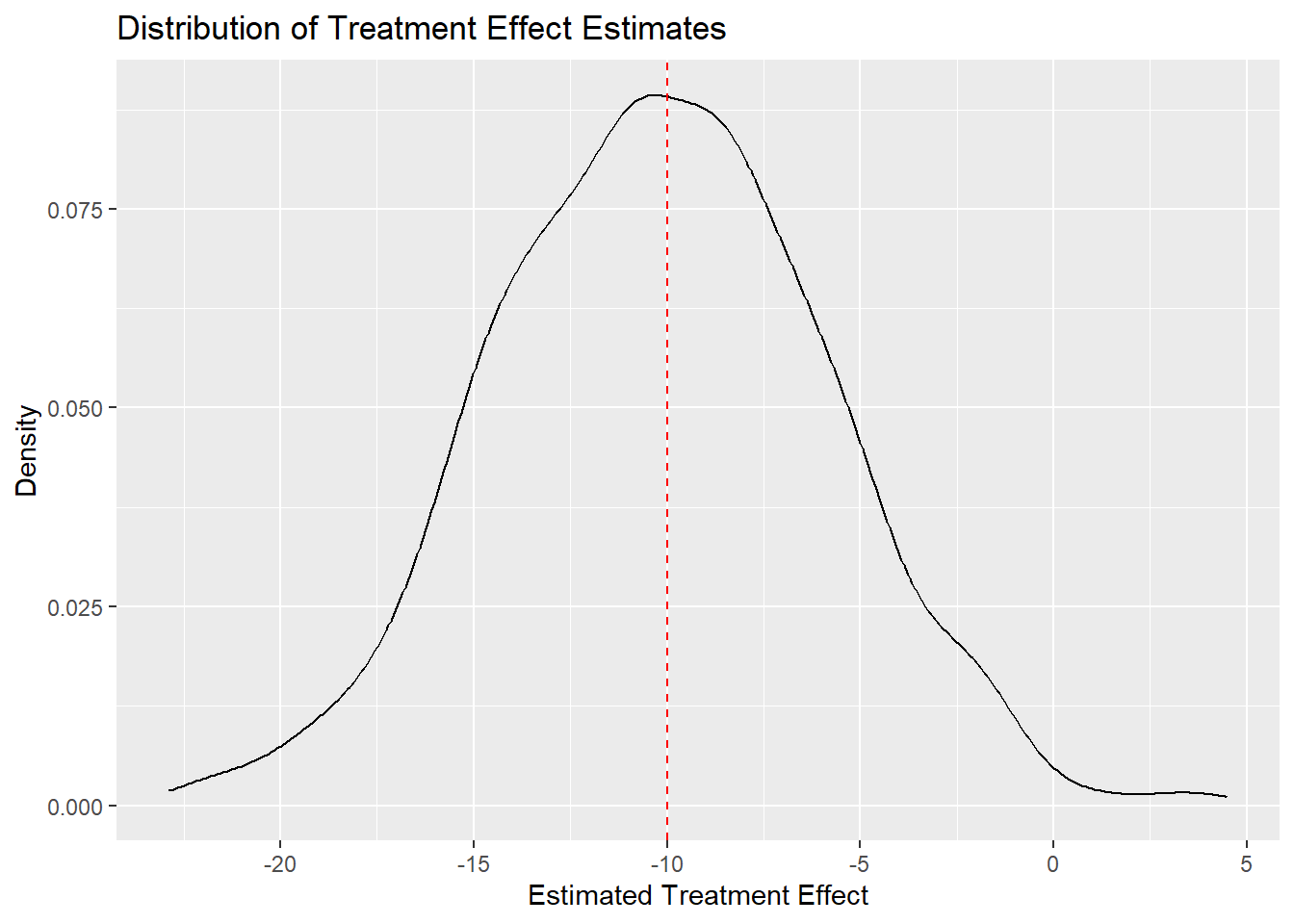
The density plot shows that the estimates are centered around the true ATE, confirming the unbiasedness of the OLS estimator in this simulation.
Wooldridge proves that the OLS estimator is unbiased for the ATE under random assignment of treatment. Our simulation is no proof, but the evidence it has generated is pretty convincing.
Note that some samples produce estimates that are quite far from the true ATE. Some estimates are below -20, while others are above 0. Which parameters of our simulation affect how tightly the estimates cluster around the true ATE? This is a question about the variance of the estimator. Think about it. We will return to it later in the course.